Basic probabilistic tractography

1.  Overview

This tutorial gives an introduction to performing basic probabilistic tractography with Camino's track command, using directional information derived from the diffusion tensor (for a guide to fitting the diffusion tensor to DW-MR image data see DTI tutorial). We will use the same human dataset used for the DTI tutorial (download).

Before starting on this tutorial, we would suggest you follow steps 1-5 of the DTI tutorial and retain all the files you create. Three additional software tools are also required for this tutorial: ITK snap, Paraview and MRIcro it might be convenient for you to download and install these now before you commence.

2.  Generating PICo Tracts

2.1  Seeding Tractography

As outlined in the basic streamline tractography tutorial, seed points are required to initiate streamlines. Here we use ITK snap to define a seed ROI in the base of the cortico spinal tract (CST):

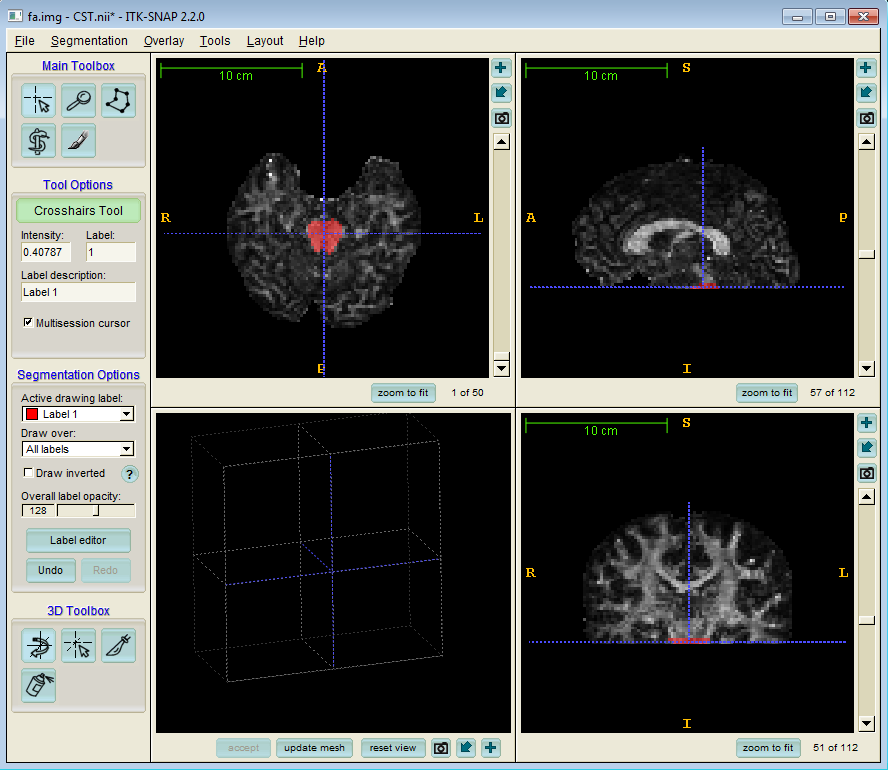
We have named our seed ROI image CST.nii.

2.2  Bayesian Tractography

Now we can use our seed ROI to generate some probabilistically tracked streamlines using bayesian tractography, the details of which are outlined in the track command page:

Here we are using the raw image data converted to voxel order format with the command:

image2voxel -4dimage 4Ddwi_b1000.nii.gz -outputfile dwi.Bfloat

as in part 4 of the DTI tutorial.

Alternatively, we can use a precomputed lookup table and PDFs:

2.3  Look-up Table and PDFs

We can use a precomputed lookup table and PDFs generated from the data and schemefile in order to execute probabilistic tracking.

Diffusion Tensor

Firstly, in order to generate the PDFs, we need to calculate the diffusion tensor in every voxel. If you haven't fit the diffusion tensor to data before, follow parts 1-5 of the DTI tutorial. We will use the dt.Bdouble file which is the output of dtfit from part 5.

Lookup table

We use the dtlutgen command to generate the look-up table:

Note here that we have set the SNR at 20, which is the SNR of this dataset. You will need to estimate the SNR of the data you are working on and set the appropriate value for the look-up table generation.

PDFs

The PICo tractography algorithm requires a probability density function (PDF) to be computed in each voxel to track probabilistically through the volume. We use the picopdfs command to generate this data:

Now we can use our seed ROI to generate some probabilistically tracked streamlines:

Note that in both cases we have defined the option -iterations 50. This means that the track command will track 50 times from each seed voxel defined in the seed ROI. This parameter can be set to any number of tracts per voxel. It's important to check test / retest reproducibility in each case, but in general we find that results are acceptably stable after 1000 iterations.

The Bayesian tractography method calculates probabilities for fiber directions directly from the DWI data in each voxel, without assuming a constant SNR or using any lookup tables. It is more data-driven than the model-based approach, and doesn't generalize easily to multiple fibre orientations, but it is more data driven. We suggest using the Bayesian method for probabilistic tractography for standard DTI acquisitions, and model-based PICo for HARDI data with multiple fiber orientations per voxel.

3.  Visualisation

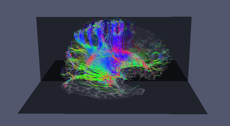
Now we can use vtkstreamlines to convert the raw streamlines into VTK streamlines and visualise them in Paraview:

4.  Maximum Connection Probability

Normally, PICo tractography is used to produce maximum connection probability maps. These maps show how likely it is for connections to exist between one voxel and another in an image.

Using the following pipeline command, we can produce connection probability maps for each voxel in the ROI:

Here, the track command produces the default 5000 tracts from each voxel in the ROI defined in CST.nii. These tracts are then processed by the procstreamlines command which produces a seperate connection probability map for each voxel in the ROI in the pico/ directory. The -outputcp option specifies that we want a connection probability map from procstreamlines.

Now we need to combine the images to form one single map for the entire ROI using imagestats

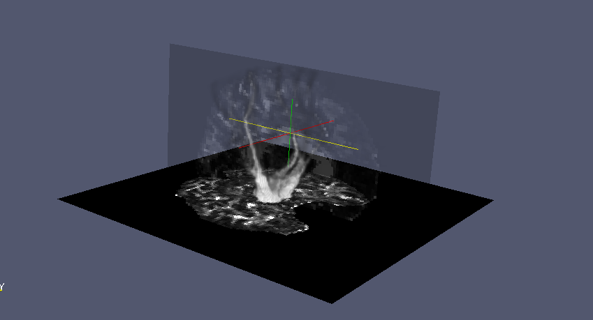
This command combines all the images for the individual ROI voxels contained in the pico/ directory into a single image roiprobs.nii which shows the maximum value found in each voxel. It should look something like the following image:

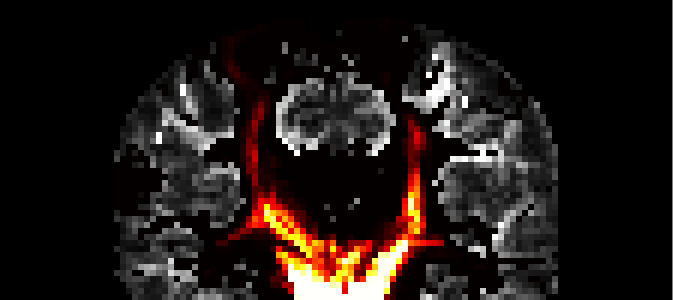
This image was created using MRIcro, the connection probability map is overlayed on the FA image.

Other statistics can also be computed with imagestats, using the options min, max, median, sum, std and var, please see the Man page for more information.

The connection probability can also be viewed in Paraview in 3D: