Basic streamline tractography

1.  Overview

This tutorial gives an introduction to performing basic streamline tractography with Camino's track command, using directional information derived from the diffusion tensor (for a guide to fitting the diffusion tensor to DW-MR image data see DTI tutorial). We will use the same human dataset used for the DTI tutorial (download).

Before starting on this tutorial, we would suggest you follow steps 1-5 of the DTI tutorial and retain all the files you create. Two additional software tools are also required for this tutorial: ITK snap and Paraview, it might be convenient for you to download and install these now before you commence.

2.  Diffusion Tensor

Firstly, in order to perform streamline tractography. We need to derive directional information for the tractography algorithm to follow. In this case, we will use the diffusion tensor. If you haven't fit the diffusion tensor to data before, follow parts 1-5 of the DTI tutorial. We will use the dt.Bdouble file which is the output of dtfit from part 5.

3.  Seeding Tractography

To track through the diffusion data, the track command requires seed points from which to initiate streamlines. These seed points are defined in an image that is in the same physical space as the diffusion data, but not always in the same voxel space. For example, your seed image could be of 1mm resolution, while your diffusion data is of 2mm resolution. But the physical space of both images should be aligned, even though the voxel indices are not.

In this tutorial, we will define seed points in the same space (same voxels, same physical space) as the diffusion tensors, specifically by drawing on the FA map derived from the DT data. By default, track will assume that the diffusion data and the seed image are in the same space.

We use the ITK snap imaging tool to define a ROI in the middle of the corpus callosum:

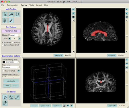
The ROI should be saved as a NifTi (.nii) file. In this example the file is named cc.nii.gz.

4.  Deterministic Tractography

Now using the ROI we have defined and the diffusion tensor data from the dtfit command, we can do some deterministic tractography using the track command:

track -inputmodel dt -seedfile cc.nii.gz -anisthresh 0.2 -curvethresh 60 -inputfile dt.Bdouble > CCtracts.Bfloat

5.  Exporting streamlines to other file formats

The .Bfloat file produced by track is a raw binary file containing all the streamlines, as documented here. They can be processed and converted to images with procstreamlines. Tract-based statistics (eg, the average FA along a streamline) can be computed with tractstats.

Streamlines can exported to VTK polydata format with vtkstreamlines.

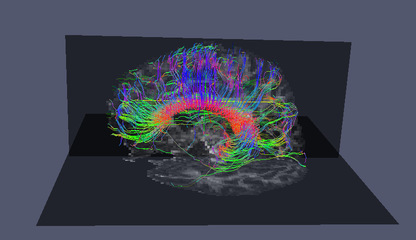
6.  Visualisation example

Paraview is one tool that can read VTK polydata as well as NIfTI images. Before we can visualise the streamlines in Paraview we need to convert the streamlines from raw format into a format that Paraview can load natively.

vtkstreamlines -colourorient < CCtracts.Bfloat > CCtracts.vtk

Here we have converted the tracts stored in raw format in CCtracts.Bfloat into tracts stored in the VTK streamlines format in CCtracts.vtk. Now the .vtk file can be loaded in Paraview for visualisation: