Multi-fibre/HARDI Reconstruction

1.  Overview

This tutorial deals with reconstruction of diffusion MRI data using multiple-fibre algorithms and voxel classification. We start by looking at the multi-tensor model of diffusion and the use of voxel classification as a way of improving the procedure. We then go on to look at multiple fibre reconstructions (specifically QBall and PASMRI) and the Camino functions that can be used to extract useful information/statistics from them.

Multiple fibre reconstruction can be quite time consuming. Therefore, prior to attempting a multiple-fibre reconstruction, we highly recommend checking the data for artefacts and other problems and then fitting the diffusion tensor (see diffusion tensor imaging tutorial) to make sure that there are no issues with scheme file. You should only proceed when you are completely satisfied that the data and schemefile are in order.

An example human data set is available for download. To pre-process the data set for this tutorial, please follow steps 1 through 5 in the diffusion tensor imaging tutorial.

2.  Voxel Classification

The command voxelclassify classifies each voxel as isotropic, anisotropic Gaussian or non-Gaussian using the algorithm in [Alexander, Barker and Arridge, MRM, Vol 48, pp 331-340, 2002]. In isotropic and anisotropic Gaussian voxels, the diffusion tensor model works well. Non-Gaussian voxels are likely fibre crossings where the diffusion tensor fails. The algorithm requires you to select thresholds for separating the three classes. First run:

voxelclassify -inputfile dwi.Bfloat -bgthresh 200 -schemefile 4Ddwi_b1000_bvector.scheme -order 4 > dwi_VC.Bdouble

To choose thresholds, run the vcthreshselect program giving it the output of the command above:

vcthreshselect -inputfile dwi_VC.Bdouble -datadims 112 112 50 -order 4

A window appears that looks like this:

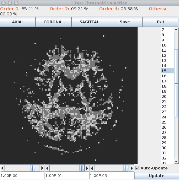
Black voxels are isotropic ("Order 0") or background, dark gray are anisotropic Gaussian ("Order 2") and light gray are non-Gaussian ("Order 4"). The light gray ones are likely fibre crossings. Scroll through the slices using the list on the right. Set the thresholds using the scroll bars or text fields at the bottom. At good threshold settings, the order 4 voxels should be fairly clustered, ie as few isolated order 4 voxels as possible with still a reasonable fraction of order 4 voxels overall. Around 5 to 10 percent order 4 voxels is typically about right.

Once you have chosen thresholds, make a note of them and generate the classified volume using voxelclassify with specified thresholds:

voxelclassify -inputfile dwi.Bfloat -bgthresh 200 -schemefile 4Ddwi_b1000_bvector.scheme -order 4 -ftest 1.0E-09 1.0E-01 1.0E-03 > dwi_VC.Bint

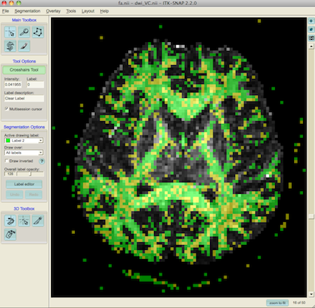
The output of this command has type int and every voxel contains either -1 for background or 0, 2 or 4 indicating the classification order. We can convert the results to NIfTI format and overlay them on the FA map using ITK SNAP:
voxelclassify -inputfile dwi.Bfloat -bgthresh 200 -schemefile 4Ddwi_b1000_bvector.scheme -order 4 -ftest 1.0E-09 1.0E-01 1.0E-03 > dwi_VC.Bint

cat dwi_VC.Bint | voxel2image -inputdatatype int -header fa.nii.gz -outputroot dwi_VC
itksnap -g fa.nii.gz -s dwi_VC.nii.gz

This shows order 2 voxels as green and order 4 as yellow.

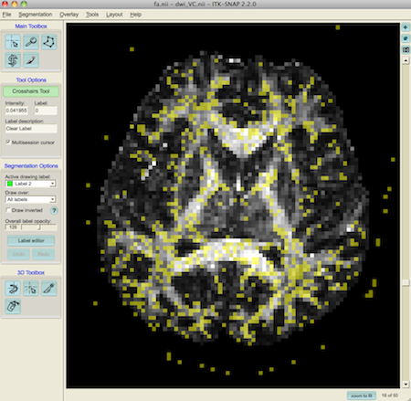
To show just the fibre crossings, we can hide label 2 using the label editor (on the left of the window)

3.  Multi-tensor

The commands modelfit and multitenfit can both be used to fit the multi-tensor model of diffusion. The modelfit command is very similar to the command used to fit the diffusion tensor. For example,

modelfit -inputfile dwi.Bfloat -inversion 31 -schemefile 4Ddwi_b1000_bvector.scheme -bgmask brain_mask.nii.gz > TwoTensorCSymA.Bdouble

or the equivalent

modelfit -inputfile dwi.Bfloat -model pospos ldt -schemefile 4Ddwi_b1000_bvector.scheme -bgmask brain_mask.nii.gz > TwoTensorCSymA.Bdouble

fits a two-tensor model of diffusion and constrains the tensors to be positive-definite. Next, dteig can then be used to calculate the eigenvectors and eigenvalues of both tensors:

dteig -inputmodel multitensor -maxcomponents 2 < TwoTensorCSymA.Bdouble > TwoTensorCSymA_Eigs.Bdouble

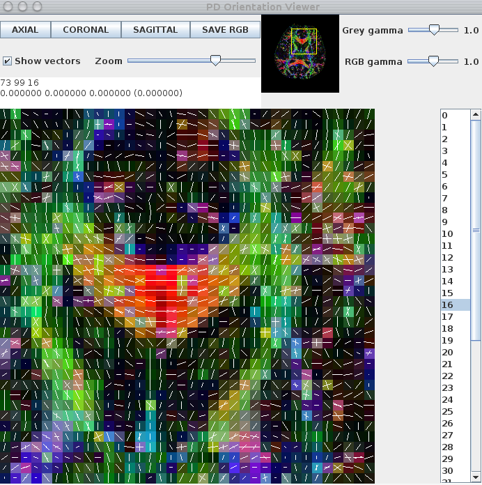
The two additional flags in dteig indicate that the model of diffusion is the multi-tensor model with a maximum of two tensors. To view the principal eigenvectors of two tensor fit, run the command

pdview -inputmodel dteig -maxcomponents 2 -datadims 112 112 50 -voxeldims 2 2 2 < TwoTensorCSymA_Eigs.Bdouble

A window appears that looks like this:

Although the two-tensor model produces a reasonable output in multiple-fibre voxels, the fit in single-fibre voxels is misleading. For example, the genu of the corpus callosum contains fibre-orientation estimates that do not reflect the underlying fibre-orientation. The reconstruction can be improved by using voxelclassify to determine whether a single-tensor or two-tensor model should be fit on a voxel-by-voxel basis. To do this, we use the voxel classification generated in Voxel Classification section, above, in the multitenfit command:

multitenfit -inputfile dwi.Bfloat -bgmask brain_mask.nii.gz -schemefile 4Ddwi_b1000_bvector.scheme -voxclassmap dwi_VC.Bint > multitensor.Bdouble
dteig -inputmodel multitensor -maxcomponents 2 < multitensor.Bdouble > multitensor_Eigs.Bdouble
pdview -inputmodel dteig -maxcomponents 2 -datadims 112 112 50 -voxeldims 2 2 2 < multitensor_Eigs.Bdouble

commands above should produce an output that looks like this:

sfplot can be used to generate images of the multi-tensor reconstructions, as opposed to just the principal orientations. To do this, we first need to split both multitensor.Bdouble and fa.img into slices. For this step we use the UNIX split command:

split -b $((112*112*17*8)) multitensor.Bdouble splitBrain/dwi_multitensor_slice
split -b $((112*112*8)) fa.img splitBrain/fa_slice

Once the data has been split into slices, we can use sfplot to generate an image:

sfplot -inputmodel multitensor -maxcomponents 2 -projection 1 -2 -xsize 112 -ysize 112 -minifigsize 30 30 -minifigseparation 2 2 -minmaxnorm -dircolcode -backdrop splitBrain/fa_slicear < splitBrain/dwi_multitensor_slicear > dwi_multitensor_slicear.rgb

In the command above, the -projection 1 -2 flag is used to flip the y-direction for the ODFs, ensuring that they are displayed in the correct orientation. The -minmaxnorm flag normalises the ODF to exaggerate its peaks.

To view the image on a UNIX machine with Image Magick installed, use the command display -size 3584x3584 dwi_multitensor_slicear.rgb (some versions of ImageMagick may require the flag -depth 8 in addition to the -size 3584x3584 flag). The file extension directly affects how display reads the file. Alternatively, you can use the ImageMagick convert command to convert dwi_multitensor_slicear.rgb to a png or other common image formats. For those that are not using UNIX, the file can be loaded into matlab using the following command:

fid = fopen('dwi_multitensor_slicear.rgb','r','b');
data=fread(fid,'unsigned char');% image in format [r_1, g_1, b_1, ..., r_N, g_N, b_N]
fclose(fid);
image=reshape(data,3, 3584,3584);
image=uint8(permute(image, [2 3 1])); % need the matrix to be in the format [x, y, rgb channel]
imshow(image,[]);
imwrite(image,'dwi_multitensor_slicear.png','png');

4.  QBall

The first stage required for QBall reconstruction is the generation of the QBall reconstruction matrix. This matrix transforms the data from a sphere in q-space to the ODF. To calculate the QBall reconstruction matrix we use qballmx:

@qballmx -schemefile 4Ddwi_b1000_bvector.scheme > qballMatrix.Bdouble

This command uses sensible defaults for the various parameters of the QBall algorithm and is equivalent to

qballmx -schemefile 4Ddwi_b1000_bvector.scheme -basistype rbf -rbfpointset 246 -rbfsigma 0.2618 -smoothingsigma 0.1309 > qballMatrix.Bdouble

The extra options can be changed to adapt the behaviour of the algorithm, see [1,2] for details. If the program has run successfully, you will see information about the basis functions used as well as their settings on the command console. Record this information for future reference as you will need it later.

We can check that the settings (i.e. the number ODF basis functions and their widths) give reasonable results by generating some test ODFs using synthetic data from datasynth using the commands

datasynth -testfunc 3 -schemefile 4Ddwi_b1000_bvector.scheme -snr 16 -voxels 10 > testData.Bfloat
linrecon testData.Bfloat 4Ddwi_b1000_bvector.scheme qballMatrix.Bdouble -normalize > testODF.Bdouble

To visualize this test data, we can create a basic greyscale image using sfplot:

sfplot -inputmodel rbf -rbfpointset 246 -rbfsigma 0.2618 -xsize 1 -ysize 10 -minifigsize 60 60 -minifigseparation 1 1 -minmaxnorm < testODF.Bdouble > testODF.gray

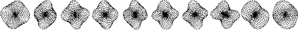
To view the image, either use the UNIX display command display -size 610x61 testODF.gray or load the data into matlab using the following command:

>> fid = fopen('testODF.gray','r','b');
>> data=fread(fid,'char');
>> fclose(fid);
>> image=uint8(reshape(data,610,61));
>> imshow(image,[]);

Once you have found settings that give reasonable results, you calculate the ODFs for each voxel of the human brain dataset using:

linrecon dwi.Bfloat 4Ddwi_b1000_bvector.scheme qballMatrix.Bdouble -normalize -bgmask brain_mask.nii.gz > dwi_ODFs.Bdouble

We choose the value for -bgthresh by thresholding the b0 image such that the background is masked while brain voxels remain. Use any image viewer (for example MRIcro, ITKsnap, Matlab or FSLView) to compare foreground and background intensities in the b0 image and pick a value that lies between the two.

To create a colour-coded image using sfplot, you first need to split the data into slices. As before, we will use the UNIX split command:

split -b $((112*112*(246+2)*8)) dwi_ODFs.Bdouble splitBrain/dwi_ODFs_slice
split -b $((112*112*8)) fa.img splitBrain/fa_slice

To create a colour-coded image, we add the flag -dircolcode. The sfplot command in full is:

sfplot -inputmodel rbf -rbfpointset 246 -rbfsigma 0.2618 -xsize 112 -ysize 112 -minifigsize 30 30 -minifigseparation 2 2 -minmaxnorm -dircolcode -projection 1 -2 -backdrop splitBrain/fa_slicear < splitBrain/dwi_ODFs_slicear > dwi_ODFs_slicear.rgb

This image can be viewed in display using the same command as before, i.e display -size 3584x3584 dwi_ODFs_slicear.rgb. In Matlab, use the commands

>> fid = fopen('dwi_ODFs_slicear.rgb','r','b');
>> data=fread(fid,'unsigned char');% image in format [r_1, g_1, b_1, ..., r_N, g_N, b_N]
>> fclose(fid);
>> image=reshape(data,3, 3584, 3584);
>> image=uint8(permute(image, [2 3 1]));\\ % need the matrix to be in the format [x, y, rgb channel]
>> imshow(image,[]);

Camino also implements the spherical harmonic (SH) QBall reconstructions of Descoteaux [3] and Mukherjee [4]. We will now create an SH representation of the QBall ODFs and use sfpeaks to find the peaks of the ODF in each voxel, which we will view in pdview. sfpeaks is a program that finds a wide range of features for any multiple-fibre reconstruction (such as PASMRI, QBall, Spherical Deconvolution). In particular, for any given voxel it outputs the number of peaks found, the mean of the function, the orientations and strengths of the peaks as well as the Hessian (or matrix of second partial-derivatives, which describes the curvature of the peak in two orthogonal directions) of each peak. This information is used in several Camino programs, including the tractography and statistics programs. To create a spherical harmonic representation of the ODF, you will need to calculate a new QBall matrix with the flag -basistype sh and then run linrecon. The full commands are:

qballmx -schemefile 4Ddwi_b1000_bvector.scheme -basistype sh -order 6 > qballMatrix_SH6.Bdouble
linrecon dwi.Bfloat 4Ddwi_b1000_bvector.scheme qballMatrix_SH6.Bdouble -normalize -bgmask brain_mask.nii.gz > dwi_ODFs_SH6.Bdouble

The command to run sfpeaks is:

sfpeaks -inputmodel sh -order 6 -numpds 3 < dwi_ODFs_SH6.Bdouble > dwi_ODFs_SH6_PDs.Bdouble

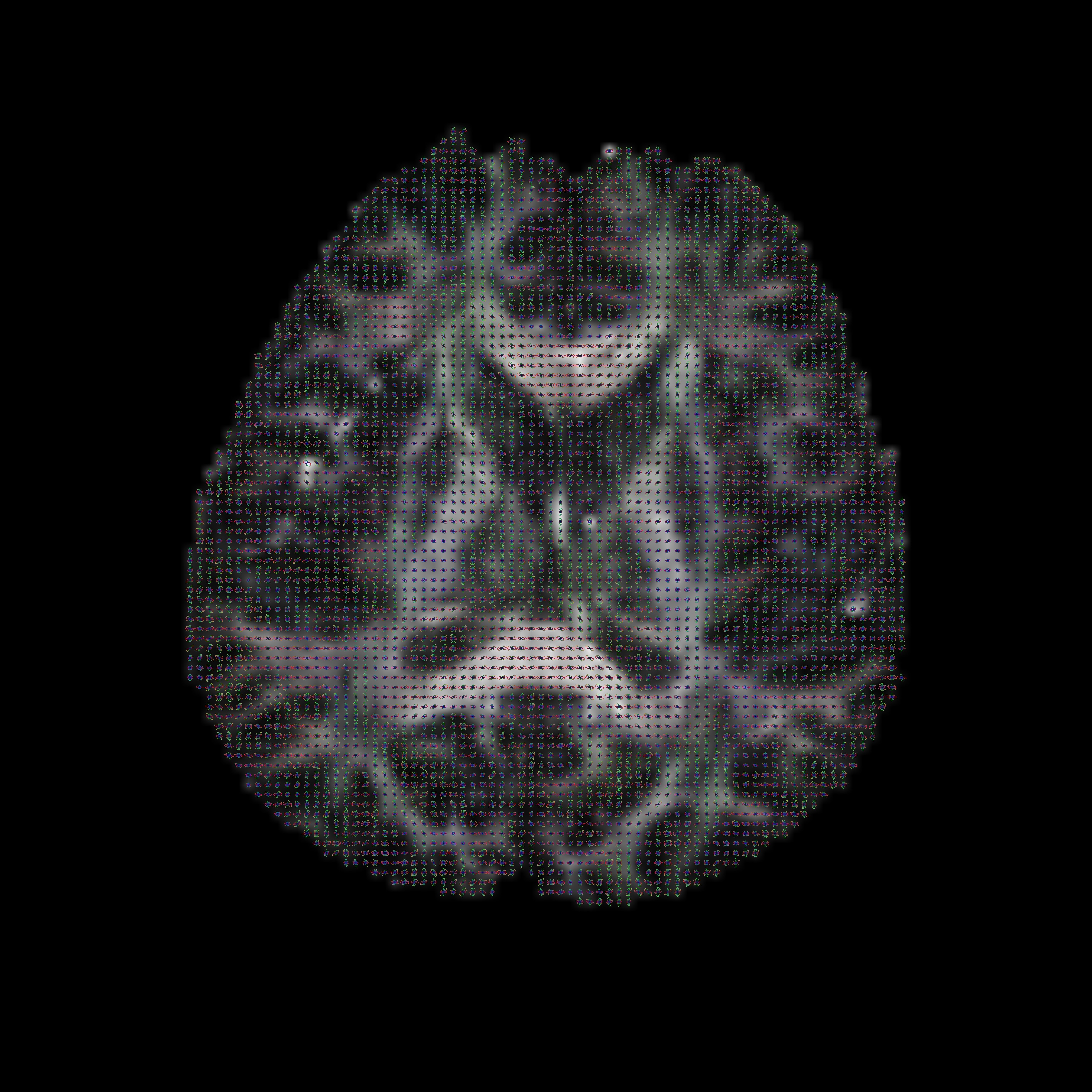
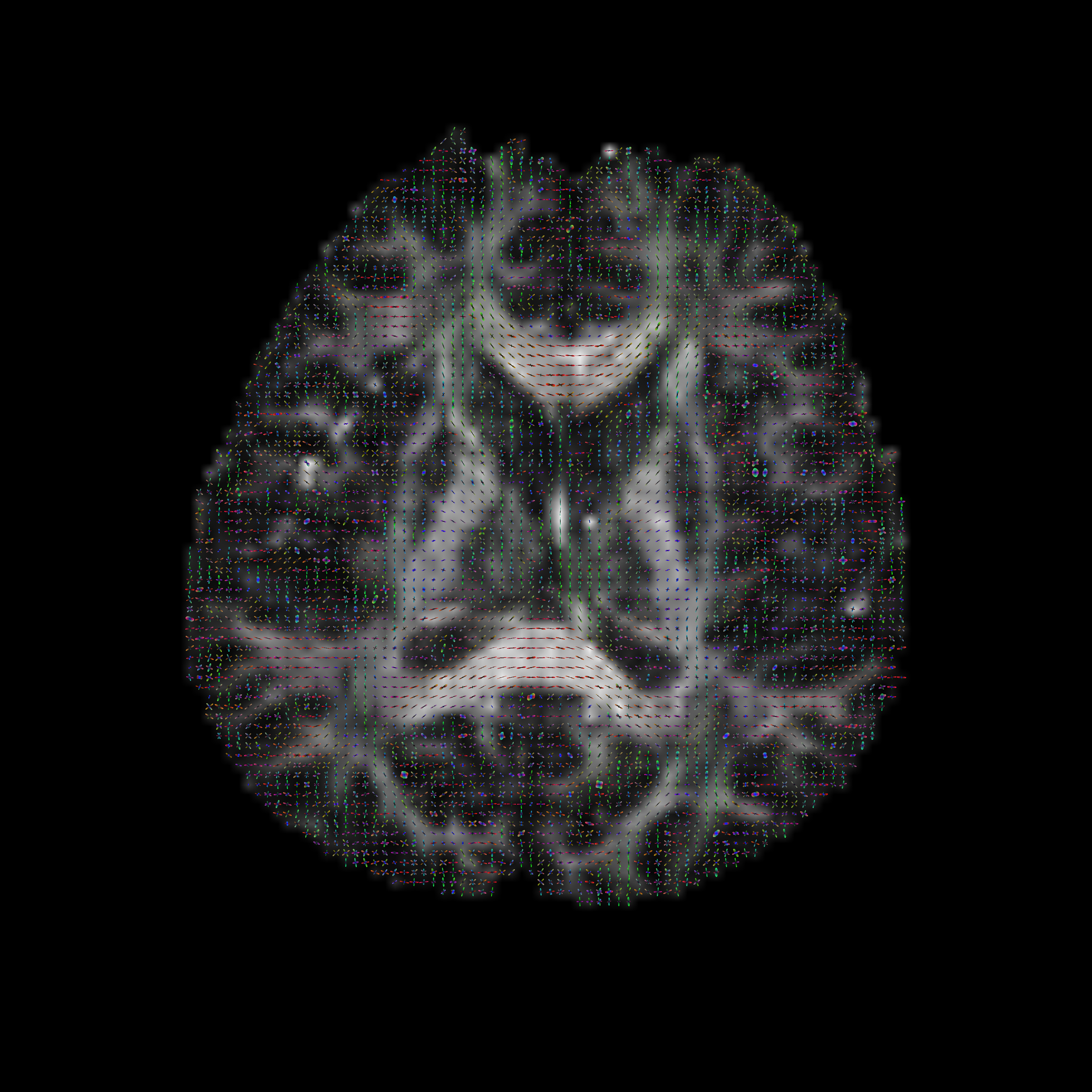
In addition to displaying the principal eigenvectors of the diffusion tensor, pdview also allows you to view the output of sfpeaks. To do this, use the flag -inputmodel pds. The background map uses the trace of the Hessian (i.e. the sharpness) of the dominant peak of each ODF. Alternatively, you can specify another greyscale background map (for example, a fractional anisotropy image) using the flag -scalarfile [filename]. The color-coding is added automatically by pdview. The command is:

pdview -inputmodel pds -numpds 3 -datadims 112 112 50 < dwi_ODFs_SH4_PDs.Bdouble

Here is an image of a pdview output:

Note that only the 2 largest peaks are displayed. The background map is generated using the trace of the Hessian, which describes peak sharpness, of the principal peak of each QBall ODF.

References

[1] D. S. Tuch. Q-Ball Imaging, Magnetic Resonance in Medicine, 52:1358-1372, 2004.

[2] D. C. Alexander. Multiple fibre reconstruction algorithms for diffusion MRI, Annals of the New York Academy of Sciences 1046:113-133 2005.

[3] M. Descoteaux. A fast and robust ODF estimation algorithm in Q-Ball imaging, Biomedical Imaging: Macro to Nano. 3rd IEEE International Symposium, 81-84, 2006

[4] C.R. Hess et al. Q-ball reconstruction of multimodal fiber orientations using the spherical harmonic, Journal Magnetic Resonance Imaging, 56:104-117, 2006.

5.  Reduced encoding PASMRI

Now lets run reduced encoding (RE) PASMRI to recover PAS functions in each voxel. The following variable, RE, specifies the number of basis functions in the PAS representation. By default, the number of basis functions is the same as the number of gradient directions. The idea of RE-PASMRI is that we can use fewer basis functions, which speeds up the estimation of the PAS. The smaller the number, the quicker the reconstruction, but the more crude the representation. Here we'll try 3 levels of reduced encoding. In practice, you'll need to experiment a bit to pick a setting that recovers crossing fibres reliably and has manageable computation time. RE=5 is probably too low, but is a good setting to use as a first run to get the whole pipeline working, as PASMRI reconstruction is fast with this low setting. RE=16 we often find is a good setting with a good trade-off between accuracy and computation time. Worth comparing with a higher setting such as RE=30 though to see whether any significant improvement occurs. To process the data, we first select a reduced encoding and run mesd:

export RE=5
#export RE=16
#export RE=30

mesd -filter PAS 1.4 -mepointset $RE -fastmesd -schemefile 4Ddwi_b1000_bvector.scheme -bgmask brain_mask.nii.gz < dwi.Bfloat > pas_1.4_me${RE}.Bdouble

In the above command, the -fastmesd flag is used to speed up the reconstruction by skipping some of the integrity checks. Once the data have been reconstructed, we use sfpeaks to find the peak orientations, which we use as our fibre-orientation estimates:

sfpeaks -inputmodel maxent -filter PAS 1.4 -schemefile 4Ddwi_b1000_bvector.scheme -mepointset $RE -numpds 3 -stdsfrommean 10 -pdthresh 1 < pas_1.4_me${RE}.Bdouble > pas_1.4_me${RE}_S10_P1_PDs.Bdouble

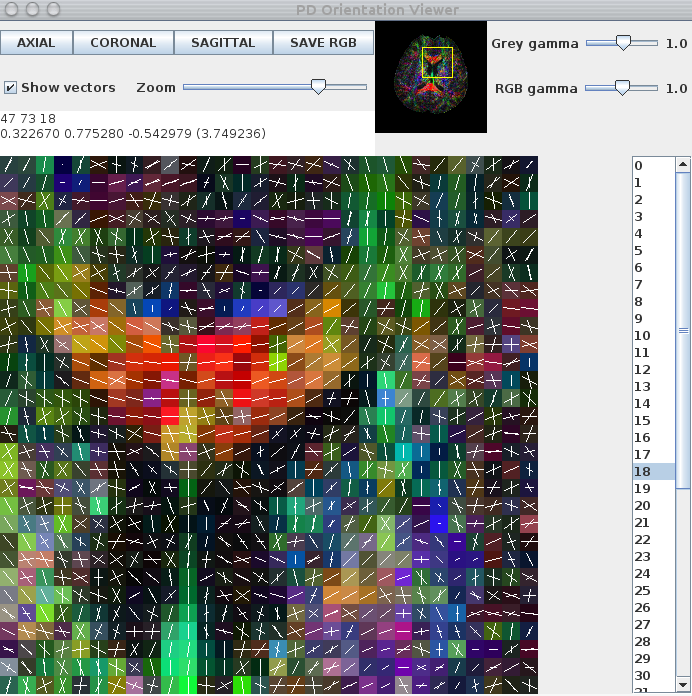
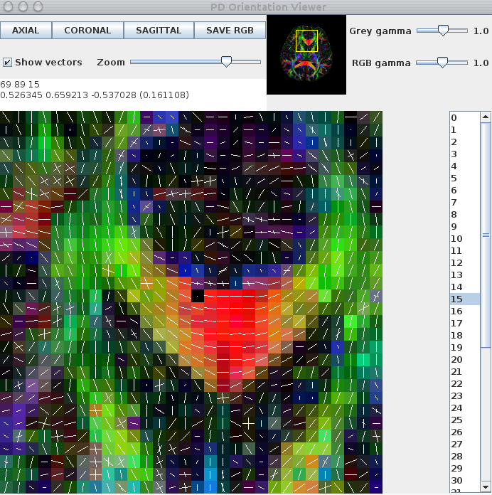
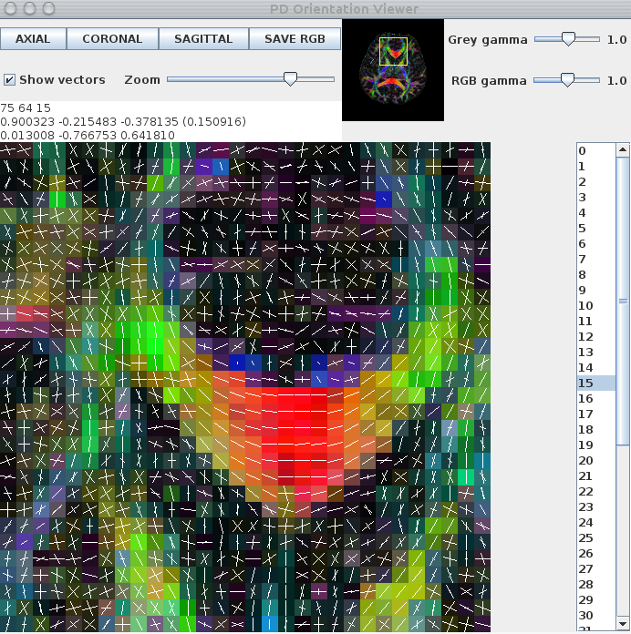
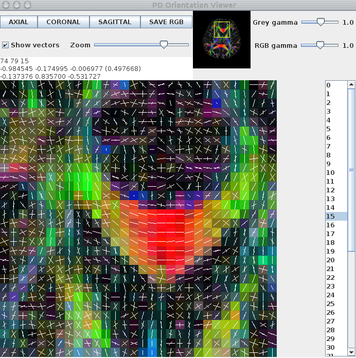
The -pdthresh and -stdsfrommean flags set thresholds for removing spurious peaks and are usually set empirically. Finally, the fibre-orientation estimates can be viewed using the pdview command

pdview -inputmodel pds -numpds 3 -datadims 112 112 50 -scalarfile fa.hdr < pas_1.4_me${RE}_S10_P1_PDs.Bdouble

The images below show a pdview screenshot for each of the reduced-encoding reconstructions (from left to right: RE=5, RE=16, RE=30). If there are voxels in white-matter that appear to have no fibre-orientation estimates (these usually show up as black squares with a white dot in the centre), you probably have the thresholds set too high. Reducing the threshold and/or removing the -fastmesd flag can improve results, although removing the -fastmesd flag can significantly increase processing times.

In addition to pdview, you can also use sfplot to generate an image for each slice of the reconstruction. We show an example sfplot command in the section on exploiting multi-core processors, below.

5.1  Exploiting multi-core processors for PASMRI reconstruction

If you have a multi-core processor, splitting the dataset into chunks and processing the data on several cores can speed up the reconstruction. In this example I am going to run the reconstruction separately for each slice, which is useful for generating nice visualizations of the results using sfplot. This directory will contain the output for each slice

# RE setting - change as required
#export RE=30; export REID=30;
#export RE=16; export REID=16;
export RE=5; export REID=05;

# Other parameter settings that need to be set (x, y and z size, number of components and dataset ID)
export XSIZE=112
export YSIZE=112
export ZSIZE=50
export COMPONENTS=33
export DSID=dwi

export mkdir PAS${REID}_${DSID}

I happen to have 8 cores, so I ran a separate process on each using the following set of 8 different for loops over the slices:

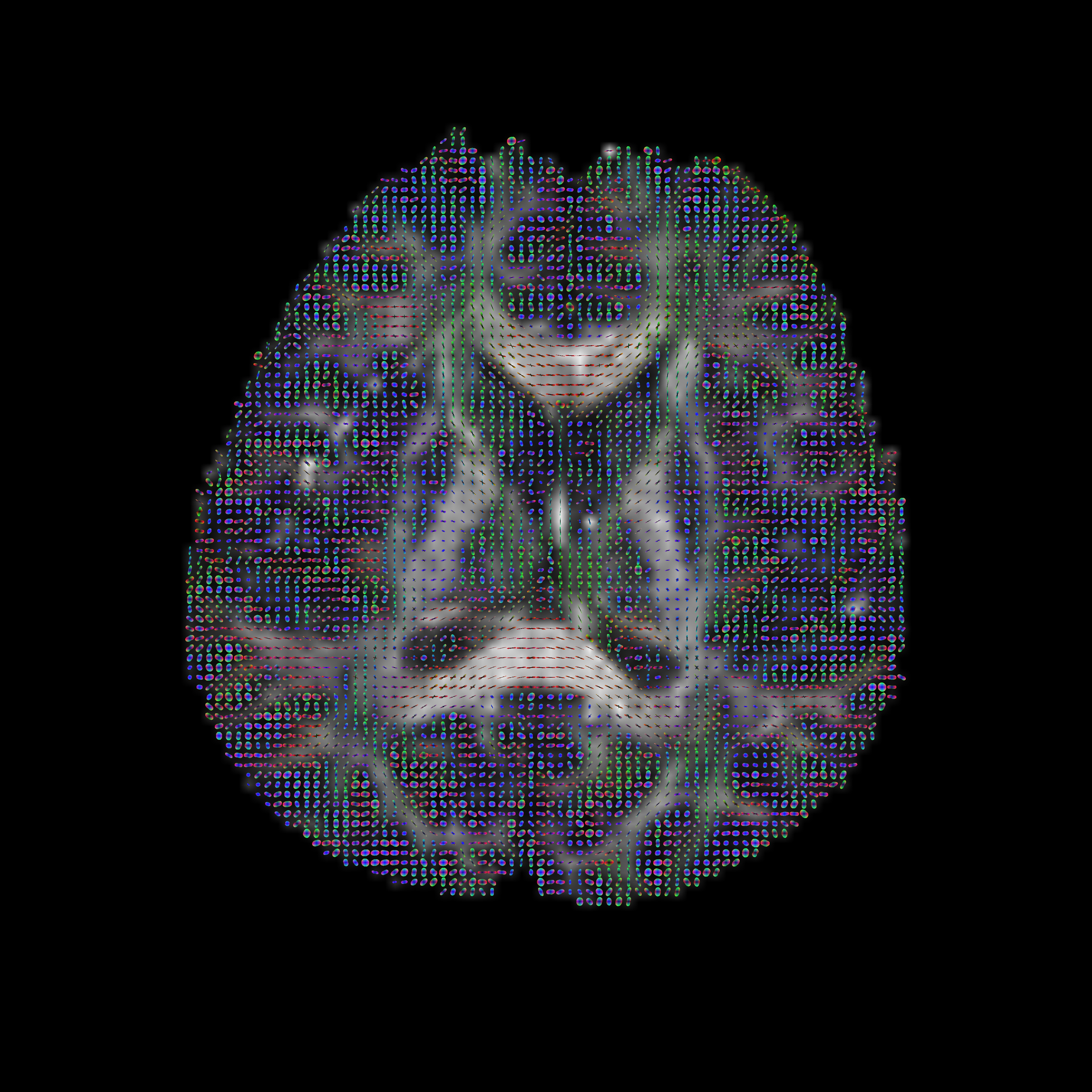
for ((i=1; i<=${ZSIZE}; i=i+8)); do
#for ((i=2; i<=${ZSIZE}; i=i+8)); do
#for ((i=3; i<=${ZSIZE}; i=i+8)); do
#for ((i=4; i<=${ZSIZE}; i=i+8)); do
#for ((i=5; i<=${ZSIZE}; i=i+8)); do
#for ((i=6; i<=${ZSIZE}; i=i+8)); do
#for ((i=7; i<=${ZSIZE}; i=i+8)); do
#for ((i=8; i<=${ZSIZE}; i=i+8)); do
echo $i
export SNUM=StringZeroPad $i 2`
shredder $((${COMPONENTS}*${XSIZE}*${YSIZE}*(i-1)*4)) $((${COMPONENTS}*${XSIZE}*${YSIZE}*4)) $((${COMPONENTS}*${XSIZE}*${YSIZE}*${ZSIZE}*4)) < ${DSID}.Bfloat > /tmp/${DSID}_Slice${SNUM}.Bfloat

dtfit /tmp/${DSID}_Slice${SNUM}.Bfloat $SCHEMEFILE | fa -outputdatatype float > /tmp/${DSID}_Slice${SNUM}_FA.img

analyzeheader -datadims ${XSIZE} ${YSIZE} 1 -voxeldims 0.5 0.5 0.5 -datatype float > /tmp/${DSID}_Slice${SNUM}_FA.hdr

mesd -schemefile $SCHEMEFILE -filter PAS 1.4 -fastmesd -mepointset $RE -bgthresh 200 < /tmp/${DSID}_Slice${SNUM}.Bfloat > PAS${REID}_${DSID}/${DSID}_Slice${SNUM}_PAS${REID}.Bdouble

sfpeaks -schemefile $SCHEMEFILE -inputmodel maxent -filter PAS 1.4 -mepointset $RE -stdsfrommean 10 -pdthresh 1 -inputdatatype double < PAS${REID}_${DSID}/${DSID}_Slice${SNUM}_PAS${REID}.Bdouble > PAS${REID}_${DSID}/${DSID}_Slice${SNUM}_PAS${REID}_PDs.Bdouble

sfplot -xsize ${YSIZE} -ysize ${XSIZE} -inputmodel maxent -filter PAS 1.4 -mepointset $RE -pointset 2 -minifigsize 30 30 -minifigseparation 2 2 -inputdatatype double -dircolcode -projection 1 -2 -pointset 5 -backdrop /tmp/${DSID}_Slice${SNUM}_FA.img < PAS${REID}_${DSID}/${DSID}_Slice${SNUM}_PAS${REID}.Bdouble > /tmp/${DSID}_Slice${SNUM}_PAS${REID}.rgb

convert -size 3584x3584 -depth 8 /tmp/${DSID}_Slice${SNUM}_PAS${REID}.rgb PAS${REID}_${DSID}/${DSID}_Slice${SNUM}_PAS${REID}.png

Here are example sfplot images for RE=5, RE=16, RE=30. Note that we use a very dense sampling pointset (-pointset 5) to capture the shape of the PAS functions. Finally, we remove the temporary files:

rm /tmp/${DSID}_Slice${SNUM}_PAS${REID}.rgb /tmp/${DSID}_Slice${SNUM}.Bfloat /tmp/${DSID}_Slice${SNUM}_FA.hdr /tmp/${DSID}_Slice${SNUM}_FA.img
done

You'll need to adapt some of the commands above for your data (specifically -voxeldims, -bgthresh and -size). You can find the script StringZeroPad in camino/SGE. convert is an ImageMagick command, which you may need to install.

Once that's all done, you can combine the results into a single file ready for tractography

cat PAS${REID}_${DSID}/*PAS${REID}_PDs.Bdouble > PAS${REID}_${DSID}/PDs.Bdouble

Now you can check that principal directions of the PAS functions:

pdview -inputmodel pds -datadims ${XSIZE} ${YSIZE} ${ZSIZE} -scalarfile ${DSID}_FA.img < PAS${REID}_${DSID}/PDs.Bdouble

6.  Multi-fibre stats

In this section, we use mfrstats to generate several useful of statistics from the output of sfpeaks. First, we generate some synthetic data, noting the test function and rotation angle used. Here we create data for 100 crossing-fibre voxels with SNR=20 using the command

datasynth -testfunc 3 -dt2rotangle 0.349 -snr 20 -schemefile 4Ddwi_b1000_bvector.scheme -voxels 100 > testData.Bfloat

Next, we reconstruct the data using reduced-encoding PASMRI and find the peaks of the reconstructions using sfpeaks:

export RE=16

mesd -filter PAS 1.4 -mepointset $RE -fastmesd -schemefile 4Ddwi_b1000_bvector.scheme < testData.Bfloat > pas_1.4_me${RE}_testData.Bdouble

sfpeaks -inputmodel maxent -filter PAS 1.4 -schemefile 4Ddwi_b1000_bvector.scheme -mepointset $RE -numpds 3 -stdsfrommean 10 -pdthresh 1 < pas_1.4_me${RE}_testData.Bdouble > pas_1.4_me${RE}_testData_PDs.Bdouble

mfrstats -voxels 100 -expect 2 -numpds 3 < pas_1.4_me${RE}_testData_PDs.Bdouble > pas_1.4_me${RE}_testData_STATS.Bdouble

double2txt < pas_1.4_me${RE}_testData_STATS.Bdouble

The output of mfrstats is in the following order:

 - number of trials (voxels in input),
 - fraction of successful trials
 - mean mean(SF)
 - std mean(SF)
 - mean std(SF)
 - std std(SF)
 - for each direction
   - mean direction (x, y, z),
   - mean dyadic eigenvalues (l1, l2, l3),
   - mean SF value,
   - std SF value,
   - mean SF largest Hessian eigenvalue
   - std SF largest Hessian eigenvalue
   - mean SF smallest Hessian eigenvalue
   - std SF smallest Hessian eigenvalue

For this example the output is:

9.300000E01 - number of trials
9.300000E-01 - fraction of successful trials
6.268984E-02 - mean mean(SF)
2.301566E-03 - std mean(SF)
8.424644E-02 - mean std(SF)
4.957507E-02 - std std(SF)
9.998178E-01 - mean x_1 -- First peak orientation
1.904221E-02 - mean y_1
1.304700E-03 - mean z_1
9.820751E-01 - mean dyadic l_1
1.487575E-02 - mean dyadic l_2
3.049180E-03 - mean dyadic l_3
2.923417E00 - mean SF value
1.716575E00 - std SF value
-1.939896E02 - mean SF largest Hessian eigenvalue
2.173765E02 - std SF largest Hessian eigenvalue
-7.642872E02 - mean SF smallest Hessian eigenvalue
9.061406E02 - std SF smallest Hessian eigenvalue
-3.187058E-01 - mean x_2 -- Second peak orientation
9.478182E-01 - mean y_2
-8.196506E-03 - mean z_2
9.859861E-01 - mean dyadic l_1
1.119527E-02 - mean dyadic l_2
2.818645E-03 - mean dyadic l_3
2.836217E00 - mean SF value
1.567252E00 - std SF value
-1.909222E02 - mean SF largest Hessian eigenvalue
2.080926E02 - std SF largest Hessian eigenvalue
-7.274968E02 - mean SF smallest Hessian eigenvalue
8.320956E02 - std SF smallest Hessian eigenvalue
0.000000E00 - -- Third peak orientation
0.000000E00
0.000000E00
0.000000E00
0.000000E00
0.000000E00
0.000000E00
0.000000E00
0.000000E00
0.000000E00
0.000000E00
0.000000E00

The output of mfrstats can be used to calculate measures of accuracy and precision, such as direction concentration and angle bias (see [1,2] for details).

Another useful tool is consfrac, which calculates the consistency fraction. This program requires a ground-truth, which in this example is given by the settings used to generate the synthetic data (namely the test function and the rotation angle of the second tensor). For a set of reconstructions to be consistent, they should have the same number of fibre-orientation estimates as the test function and the peak orientations should be within a given tolerance of the true fibre-orientation. To run consfrac, we use the command

consfrac -voxels 100 -numpds 3 -testfunc 3 -dt2rotangle 0.349 < pas_1.4_me${RE}_testData_PDs.Bdouble > pas_1.4_me${RE}_testData_CF.Bdouble

double2txt < pas_1.4_me${RE}_testData_CF.Bdouble

The output of the program is:

1.000000E02 - number of trials
1.000000E00 - fraction of successful trials
9.100000E-01 - consistency fraction
References

[1] D.C. Alexander. Maximum entropy spherical deconvolution for diffusion MRI, In Proc. Information processing in medical imaging, 2005.

[2] K.K. Seunarine and D.C. Alexander. Multiple fibers: beyond the diffusion tensor. In Diffusion MRI: from quantitative measurement to in vivo neuroanatomy. Academic Press. 2009.