
Using Camino with Human Connectome Project Data (HCP)
On this page... (hide)
Diffusion weighted data acquisitions from the WU-Minn HCP consortium are accompanied by a gradient deviation file, grad_dev.nii.gz. These files contain individual gradient field deviations at each voxel and are used to correct the gradient nonlinearities associated with the high performance gradient coils. These nonlinearities are higher than in normal 3T scanners, reaching up to 15% from their nominal value (Sotiropoulos et al. NeuroImage 2013). As a result of this, it is recommended that the corrections be applied when fitting models to the data. The following tutorial demonstrates how to perform a linear Diffusion Tensor fit in Camino with gradient nonlinearity correction for HCP data. In step 5 some short examples for other diffusion imaging models are shown.
1. Setup and Data
Before starting, you will need to increase the amount of RAM allocated to Camino from the default value of 1000Mb. To do this you must know which type of shell you are using, if you are unsure, type:
echo $SHELL
If you have a sh/bash shell then type:
export CAMINO_HEAP_SIZE=4000
If you have a csh/tcsh shell then type:
setenv CAMINO_HEAP_SIZE 4000
Note that to use the whole 3-shell HCP dataset, as is, you may need to allocate a large amount of RAM (~11000Mb) when converting the data to the Camino format (step 3 in this tutorial). Depending on your application, you may wish to instead extract single shells including b=0s/mm^2 (really b=5s/mm^2) images and the corresponding bvals and bvecs entries to fit models to a single shell at a time, as in this tutorial. This will reduce system requirements to approximately 4000Mb. This tutorial uses a single shell HCP dataset, from the 100408 subject, but the same procedure can be followed exactly for a 3-shell dataset.
You will need the following files (or the default files for a 3-shell fit):
| File | Description |
|---|---|
| data_1000.nii.gz | Raw DWI data in NIfTI-1 format for b=1000s/mm^2(approximately) and b=0s/mm^2 images only. |
| bvals_1000 | List of b - values with only b=1000s/mm^2 and b=0s/mm^2 only. |
| bvecs_1000 | List of gradient directions corresponding to b=1000s/mm^2 and b=0s/mm^2 gradients only. |
| nodiff_brain_mask.nii.gz | Binary mask separating brain from background. |
| grad_dev.nii.gz | Gradient deviation information at each voxel |
2. Create a Schemefile
The first stage of fitting a model to the diffusion data is preparing a schemefile. Currently, the schemefile used for HCP data, if you want to include gradient correction, must be a BVECTOR scheme (see schemefiles page for more information). This scheme version can be generated from the bvals and bvecs files using the fsl2scheme command.
fsl2scheme -bvecfile bvecs_1000 -bvalfile bvals_1000 > hcp.scheme
3. Convert the Data
The diffusion weighted data comes in NIfTI-1 format and must be converted to the Camino format using image2voxel.
image2voxel -4dimage data_1000.nii.gz -outputfile dwi.Bfloat
Where the output file now contains the raw diffusion weighted data in the voxel-ordered binary format that Camino uses. The file extension .Bfloat of the output file indicates that the file contains big-endian floats. Raw data produced by Camino is always big-endian. By default, most data is of type double, but DWI data is of type float. For further information. please see the data import page.
4. Fit the Diffusion Tensor
To fit the Diffusion Tensor model whilst including a gradient correction to the scheme data at each voxel, simply add the extra flag -gradadj to the usual modelfit parameters.
modelfit -inputfile dwi.Bfloat -schemefile hcp.scheme -gradadj grad_dev.nii.gz -model ldt -bgmask nodiff_brain_mask.nii -outputfile dt.Bdouble
We can now compute the fractional anisotropy (FA) and mean diffusivity (MD) maps from our diffusion tensor estimates.
for PROG in fa md; do
	cat dt.Bdouble | ${PROG} | voxel2image -outputroot ${PROG} -header data_1000.nii.gz
done
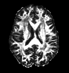
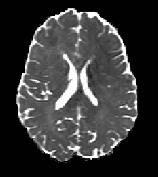
The voxel2image command above means that the FA and MD maps have been converted back into image format and can now be viewed using an external program such as Matlab. The FA(left) and MD(right) for this dataset are shown below and they correspond well to the expected FA and MD maps for DWI of human brains. For example MD shows highest diffusivity in CSF regions and FA displays highest anisotropy in white matter regions.
For more detailed information on the diffusion tensor model including how to calculate tensor orientations please refer to the DTI tutorial. Here you will also find information on how to perform a weighted linear DT fit which is more robust than the linear least squares fit used above and still supports the gradient corrections.
5. Other Models
It is currently possible to apply the gradient corrections for 3 types of fitting procedure (including the diffusion tensor model) simply by including the added flag -gradadj to the normal fitting program. The other models which support this are shown below.
i) Some compartment models using the Levenberg-Marquardt algorithm. Below is an example of this for the Ball-Stick model.
modelfit -inputfile dwi.Bfloat -fitmodel BALLSTICK -fitalgorithm MULTIRUNLM -samples 100 -schemefile hcp.scheme -voxels 1 -gradadj grad_dev.nii.gz -outputfile bs.Bdouble
see WM analytic models tutorial for more information on compartment models.
ii) For fitting the spherical harmonic series to the apparent diffusion coefficient profile.
shfit -inputfile dwi.Bfloat -schemefile hcp.scheme -gradadj grad_dev.nii.gz -order 4 -outputfile shs.Bdouble
refer to shfit page for more information on this.