

Connectivity Matrices
On this page... (hide)
1. Overview
This tutorial explains how to reconstruct connectivity matrices given a set of labeled ROIs and set of tracts. The program to compute the connectivity matrix is conmat.
The conmat command takes as input a target image containing labeled regions, and streamlines output by track. It generates a matrix counting the number of streamlines connecting each pair of labels in the target image. In a graph representation, labeled regions are nodes and the streamlines are undirected edges connecting some or all of the pairs of nodes. conmat can also compute scalar statistics along the streamlines, such as the average FA of each line connecting a pair of nodes.
The user may use any tractography algorithm supported by track and may also pre-process the streamlines with procstreamlines. Additional normalization will probably be required; for example we might want to correct the raw connectivity scores for total brain volume, or for the total number of streamlines that were generated by track. These operations must be done by the user after computing the matrix with conmat.
In this tutorial, we will walk through the use case of calculating a whole-brain cortical connectivity matrix, using a dense cortical labeling as the nodes.
2. Fiber-count connectivity matrix
The format of the output connectivity matrix is a comma separated variable (CSV) file with a one-line header containing the name of the labels and the connectivity matrix entries thereafter. This format is suitable for reading into R with the read.csv command. The column names can be passed to conmat or generated automatically based on the label intensities.
The simplest use of conmat is to create a connectivity matrix representing counts of fibers connecting one region of the atlas to the other. As an example we will use a set of labels from MindBoggle, consisting of 25 cortical regions per hemisphere, as discussed in Klein et al (2012). The labels were transferred to the DWI image used in the DTI tutorial, via an intermediate template. To run the examples in this tutorial, download the labels and associated images and the DWI data.
We first compute the streamlines that are input to conmat by calling track. We can do this with probabilistic tractography:
track -inputfile 4Ddwi_b1000.nii.gz -schemefile 4Ddwi_b1000_bvector.scheme -inputmodel bayesdirac -pointset 0 \
-iterations 10 -seedfile seeds03.nii.gz -curvethresh 75 -tracker euler -stepsize 0.5 -brainmask brain_mask.nii.gz \
-outputfile allTracts.Bfloat
This takes a while, a faster alternative is to use deterministic tracking by first fitting the diffusion tensor:
wdtfit 4Ddwi_b1000.nii.gz 4Ddwi_b1000_bvector.scheme -brainmask ../brain_mask.nii.gz -outputfile camino_wdt.nii.gz

track -inputfile camino_wdt.nii.gz -inputmodel dt -seedfile seeds03.nii.gz -curvethresh 75 -tracker euler -stepsize 0.5 \
-brainmask brain_mask.nii.gz -outputfile allTracts.Bfloat
Here we have written the output of wdtfit to a NIfTI file, which is a vector image containing the 8 components produced by wdtfit.
Generally, we are interested in connections between different labeled regions. In this case, we can reduce the output file size by piping to procstreamlines:
track -inputfile camino_wdt.nii.gz -inputmodel dt -seedfile seeds03.nii.gz -curvethresh 75 -tracker euler -stepsize 0.5 \
-brainmask brain_mask.nii.gz | procstreamlines -endpointfile kirby_mindboggle_25_warped.nii.gz \
-outputfile allEndPointTracts.Bfloat
This removes lines that don't connect a pair of diifferent labeled regions.
The results below are based on the results of probabilistic tracking, but the workflow is the same if you use deterministic tracking.
conmat -inputfile allTracts.Bfloat -targetfile kirby_mindboggle_25_warped.nii.gz -targetnamefile dkt25.csv \
-outputroot mindboggle_25_
This command creates a CSV file mindboggle_25_sc.csv containing the streamline counts (sc) connecting any pair of labeled regions. The first line of the output is the header, which contains the label names from the file dkt25.csv. If this file was not present, then the labels would be named by intensity, for example voxels with intensity 100 would be called "Label100". The matrix is symmetric since the same number of tracts connects region A to B or B to A.
The target name file can be comma or space separated. Label names should not contain commas and those with spaces should be quoted. No header line should be included.
The matrix can be visualized in many ways, for example by a heat map in R:
library(gplots)
conmat = read.csv("mindboggle_25_sc.csv")
row.names(conmat) = colnames(conmat)
heatCols = colorRampPalette(c("dark red", "red", "orange", "yellow", "white"))
x = heatmap.2(as.matrix(conmat),  Rowv=TRUE, Colv=TRUE, dendrogram = "none" , trace = "none",
margins = c(16, 16), col = heatCols, breaks = seq(5, 155, 10))
3. Using a subset of labels
The label name file can be used to define a subset of labels in the target file. Labels that do not have a name will be disregarded by conmat. For example, if we only care about left hemisphere labels, we could edit out those labels and re-run conmat. When you remove a label in this way, it is as if it doesn't exist in the target file.
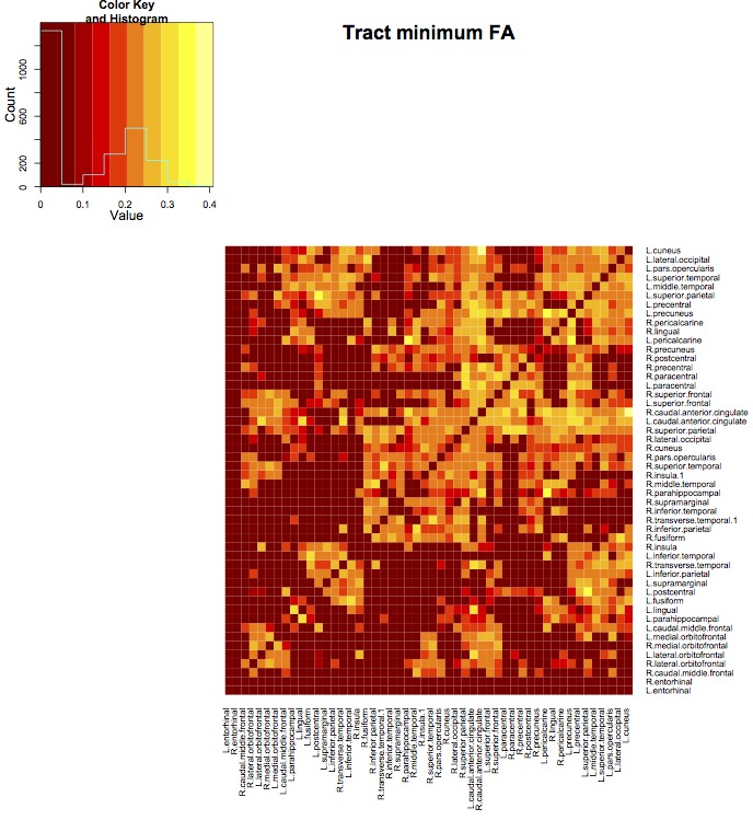
4. Tract Statistics
In addition to counting the streamlines connecting a pair of regions, conmat can calculate statistics on scalar images, computed along the tracts. These are computed in additional to the usual streamline counts.
Tract statistics are based on images in the same physical space as the streamlines. Different statistics can be computed for each streamline: mean, min, max, sum, median, var. One number is generated per streamline connecting a pair of regions, the mean of these values is entered into the matrix. For example, to get the average minimum FA along streamlines, use -tractstat min. Given a pair of regions, conmat will find the minimum FA Fmin along each streamline connecting the pair, and then place the mean of Fmin into the matrix.
fa -inputfile camino_wdt.nii.gz -outputfile fa.nii.gz
conmat -inputfile allTracts.Bfloat -targetfile kirby_mindboggle_25_warped.nii.gz -targetnamefile dkt25.csv \
-scalarfile fa.nii.gz -tractstat min -outputroot mindboggle_25_
The streamline counts are output as before, but we also get mindboggle_25_ts.csv containing the average minimum FA along streamlines connecting each pair of regions.
Two tract statistics can be used without any scalar volume, because they are intrinsic to the streamlines themselves. These are length and endpointsep (see tractstats for more information). In this case you would get the average length of paths connecting the two regions, or the euclidean distance between the end points of the paths. The ratio of these measures yields a crude measure of streamline curvature.
5. Visualization in Matlab
Matlab code for matrix visualization is provided by Michael Dayan. The functions called in the example below are available here.
conmat_path='mymatrix_sc.csv';
myconmat = csvread(conmat_path,1,0);
figure, imagesc(myconmat)