Multi Fiber Tractography

1.  Overview

Note: Parts of this tutorial are out of date. OOGL output is no longer supported, use vtkstreamlines instead and render in a VTK viewer such as Paraview.

This tutorial runs through deterministic and probabilistic tractography using multiple-fiber reconstructions like PASMRI and q-ball. I'll start with a data file of diffusion weighted measurements in Camino voxel-order format, called B4069.Bfloat, and corresponding schemefile, called B4069.scheme. The data set has 105 gradient directions with b value 4069s/mm^2 (it actually comes from a fixed brain) and 25 b=0 images. Here are the stages we'll go through: Deterministic and probabilistic DTI tractography as a baseline PAS reconstruction using reduced encoding PASMRI (see Sweet and Alexander ISMRM 2010). Deterministic tractography using PASMRI Probabilistic tractography using PASMRI q-ball reconstruction and tractography for comparison Define some variables used throughout, which are specific to my data set:

2.  DTI Tractography

This is covered in detail in other tutorials, so I'll keep it brief. Fit the diffusion tensor and check that the tensor orientations correspond with the image orientation:

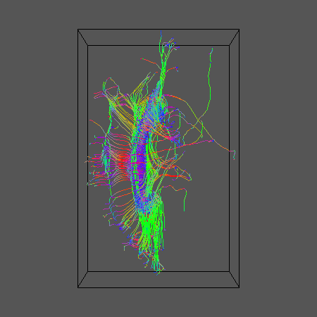
Run deterministic tractography from a seed region (mine is the midsagittal corpus callosum):

Display the tract:

Here's what we get

Now run some probabilistic tractography. Start by generating the look up table and create the pdfs in each voxel

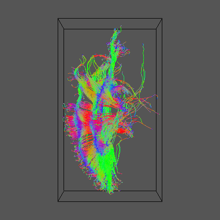
Now do the tracking (you may want to increase the number of iterations in a real application):

And display the results for comparison:

3.  Reduced-encoding PASMRI

Now lets run reduced encoding (RE) PASMRI to recover PAS functions in each voxel. The following variable, RE, specifies the number of basis functions in the PAS representation. By default, the number of basis functions is the same as the number of gradient directions. The idea of RE-PASMRI is that we can use fewer basis functions, which speeds up the estimation of the PAS. The smaller the number, the quicker the reconstruction, but the more crude the representation. Here we'll try 3 levels of reduced encoding. In practice, you'll need to experiment a bit to pick a setting that recovers crossing fibres reliably and has manageable computation time. RE=5 is probably too low, but is a good setting to use as a first run to get the whole pipeline working, as PASMRI reconstruction is fast with this low setting. RE=16 we often find is a good setting with a good trade-off between accuracy and computation time. Worth comparing with a higher setting such as RE=30 though to see whether any significant improvement occurs.

I'm going to run the reconstruction separately for each slice, which is useful for generating nice visualizations of the results using sfplot. This directory will contain the output for each slice mkdir PAS${REID}_${DSID}@] If you only have one processor, use the following for loop (or just run the whole file in one go):

I happen to have 8, so I ran a separate process on each using the following set of 8 different for loops over the slices:

You'll need to adapt some of the commands above for your data (specifically -voxeldims, -bgthresh and -size). You can find the script StringZeroPad in camino/SGE. convert is an ImageMagick command, which you may need to install.

Once that's all done, you can combine the results into a single file ready for tractography

Now you can check that principal directions of the PAS functions:

4.  PAS Tractography

Deterministic tractography:

For comparison with DT results:

Here are results for RE=5, 16 and 30:

Now try some probabilistic tractography. Start by calibrating the pdf generator. This command creates a full size calibration data set (see sfpicocalibdata man page):

For my postmortem data set, I had to add -trace 8E-10, to specify a lower diffusivity for fixed tissue at room temperature than the default, which is meant for in-vivo tissue. I've removed it from the above so in-vivo users can cut and paste. I've used -snr 12, as the signal to noise of my unweighted images is around 12. Performance is reasonably robust to this setting so don't worry if the SNR varies over the image. Just pick a ball park correct figure. Now do the actual calibration. This involves running RE-PAS on the calibration data set and constructing a look-up table. Over the full calibration data set, even RE-PAS can take a while. To get a quick set of results for a first pass, have a look at the sfpicocalibdata man page to see how you can reduce the size of the data set. You may find that you need to add arguments like -binincsize 2 -minvectsperbin 10 to sflutgen below to get it to work on smaller calibration data sets; check the sflutgen man page to see what they do. If you find you need such arguments for the full calibration data set, the calibration data set is not large enough. Anyway, here goes...

Note that the above uses a Watson model for the pdfs. You can also use Bingham; see sflutgen man page.

Now we can get the pdfs and do the tracking:

Results for R=5, 16 and 30 as before:

5.  Q-ball reconstruction and tractography

Do the q-ball reconstruction using spherical harmonic representation up to order 6:

Note the sfpeaks command can take quite a while.

Check the directions are OK:

Do some deterministic tractography:

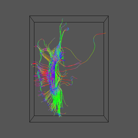
Using the same calibration data set constructed above for PAS-PICo, calibrate for q-ball PICo

Get the pdfs and run the tractography: