Monte-Carlo Mesh Simulation

1.  Overview

This tutorial describes how to run Monte-Carlo diffusion simulations on mesh substrates. This is the most flexible and realistic type of substrate currently supported by the simulation. Mesh substrates model the environment as a collection of triangles and as such can model almost any shape in three dimensions. Mesh substrates have been successfully used to simulate diffusion in environments constructed from highly complex micrograph images (Panagiotaki et al, 2010), and validate assumptions on white matter models with orientation dispersion where analytic expressions are unavailable (Wang et al, 2013).

2.  Simulation on meshes

This section describes some of the main assumptions made about mesh substrates, techniques used in the simulation, and the format of files used to store meshes.

The size of a substrate is determined by the minimum and maximum values in x, y and z dimensions. The simulation then creates a cuboidal bounding box to fully accommodate the substrates. The space within the bounding box is divided into two parts: intracellular space, the portion inside the substrate, and extracellular space, the portion outside the substrate. The bounding box has limited size, but spin may diffuse beyond it when the substrate size is relatively small and diffusion time is long. We assume that all substrates have periodic boundaries. By doing this, when spins diffuse beyond the boundaries of bounding box, it re-enters the box on the opposite side. To make this periodicity assumption sensible, we encourage constructing substrates with matching boundaries (Hall and Alexander, 2009; Wang et al, 2013). However, when the meshes becomes complicated, such as the one reconstructed from asparagus images in Panagiotaki et al 2010, it can be very difficult to construct periodic boundaries. The spins near the boundaries of the bounding box do not experience a constant environment, thus may produce meaningless signals. Our solution is to discard spins near the boundaries, and collect signals only from these near the centre, which are exposed in a relatively constant environment. The fraction between the area where signals are to be collected and the total area of the bounding box is called voxel size fraction (voxelsizefrac). The optimal fraction for the substrates in Panagiotaki et al 2010 is 0.75, which is now used as the default value for mesh substrates in the simulation. As the substrate is periodic, two faces in the opposite side can appear very close to each other, which may potentially cause numerical problems. To avoid this, we allow users to customise separation between bounding boxes when needed.

It is not compulsory to use triangles to generate mesh files, because the simulation will automatically triangulate them if they are not. Meshes are stored and defined via a simple file format called PLY. A PLY files consists three main parts: header, vertices and faces. Here are the contents of a simple PLY file of the type the simulation prefers:

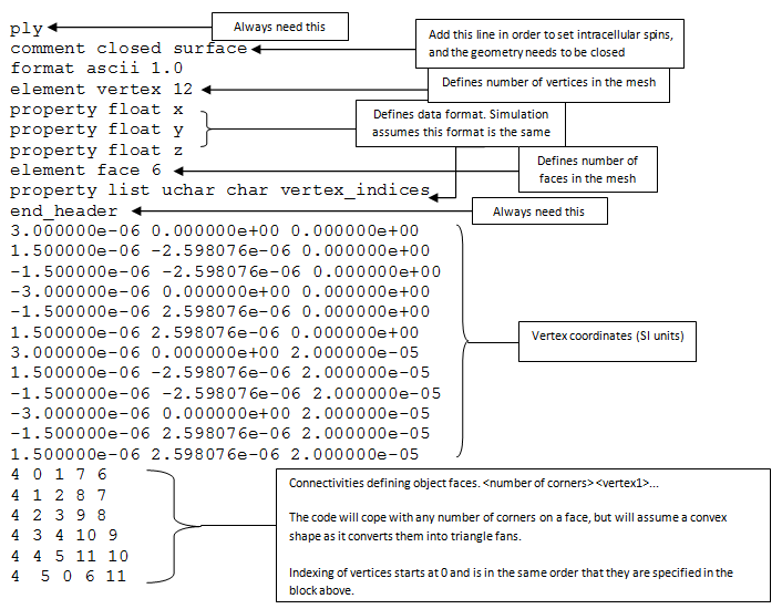
Because meshes can have arbitrary structure, they do not have a default intracellular or extracellular space. To distinguish the two spaces, the geometry needs to be closed, and ‘comment closed surface’ must be added in the header of the PLY file to inform the simulation about this. To determine the two spaces, the ray-test algorithm is used. A ray is projected from the position of a spin to an arbitrary direction. Then the number of intersections between the ray and the mesh faces is counted, an odd number of intersections indicate an intracellular spin, otherwise, it is an extracellular one. This can be important during simulation initialisation. If we specify intracellular spins, it will be a ‘trial and error’ procedure. The program picks a random position, checks whether it is intracellular. If it is, then take it; otherwise pick another random position. Be aware that it may take long time to get all spins initialised in the intracellular space when substrate has a low intracellular volume fraction.

3.  Simulation examples

In this section, we show two examples of running Monte-Carlo mesh simulations. The simulation command is datasynth, exactly the same as any other substrate. We need to use the option -substrate ply, together with -plyfile to specify the name of the PLY file. The separation between bounding box for mesh substrates can be specified by –meshsep, which is similar to -cylindersep in cylinder substrates.

3.1  Regular cylinder Vs polygon mesh cylinder

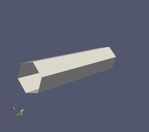
In this example, we will compare synthetic signals from polygon mesh cylinders with regularly packed cylinders (regCyl), to investigate how much discretization of a circular cylinder affects signal accuracy. We construct polygon mesh cylinders by discretizing a circular cylinder cross section into six and twelve vertices, named cyl6 and cyl12 respectively. All cylinders have radius 3E-6m. Mesh cylinders are parallel to z-direction and have length 25E-6m. Below shows Paraview images of cyl6 (left) and cyl12 (right), and the PLY files can be downloaded here.

In this example, we will use the scheme myScheme.scheme1, which contains 80 b = 9542 s/mm2 measurements with gradient directions uniformly distributed in a sphere. We define a variable to store the name of the scheme file.

schemefile="myScheme.scheme1"

Now we will start the simulation. First, we synthesize signals from regularly packed cylinders.

 
N=100000	# number of spins
T=10000	        # number of updates

r=3E-6	        # cylinder radius
sep=6.1E-6	# cylinder seperation
outputfile="regCyl_r=3E-6_spike.Bfloat"	# name of the output file

datasynth -walkers ${N} -tmax ${T} -p 0.0 -voxels 1 -initial spike -voxelsizefrac 1 -diffusivity 0.6E-9 \
-schemefile ${schemefile} -substrate cylinder -packing square cylinderrad ${r} -cylindersep ${sep}\
 -outputfile ${outputfile} 

Second, we synthesize signals from mesh cylinders. We first specify cylinder separations, such that the intracellular volume fractions match that in regularly packed cylinder substrates.

xsep=6.1E-6      # the same separation as regCyl
ysep=6.1E-6	 # the same separation as regCyl
zsep=25E-6	 # this need to match the height of the mesh cylinder

Then the following commends generate the synthetic signals.

# synthesizes signals for cyl6.
plyfile="cyl6_r=3E-6.ply"
outputfile="cyl6_r=3E-6_spike.Bfloat"
datasynth -walkers ${N} -tmax ${T} -p 0.0 -voxels 1 -initial spike -voxelsizefrac 1 -diffusivity 0.6E-9 \
-meshsep ${xsep} ${ysep} ${zsep} -schemefile ${schemefile} -substrate ply -plyfile ${plyfile} \
-outputfile ${outputfile}

# synthesizes signals for cyl12.
plyfile="cyl12_r=3E-6.ply"
outputfile="cyl12_r=3E-6_spike.Bfloat"
datasynth -walkers ${N} -tmax ${T} -p 0.0 -voxels 1 -initial spike -voxelsizefrac 1 -diffusivity 0.6E-9 \
-meshsep ${xsep} ${ysep} ${zsep} -schemefile ${schemefile} -substrate ply -plyfile ${plyfile} \
-outputfile ${outputfile}

After simulation, we can plot the signals using the following MATLAB code.

% load signals.
signalfName = 'regCyl_r=3E-6_spike.Bfloat';
fid = fopen(signalfName, 'r', 'b');
regCyl = fread(fid, 'float'); % synthetic signals from regCyl.
fclose(fid);

signalfName = 'cyl6_r=3E-6_spike.Bfloat';
fid = fopen(signalfName, 'r', 'b');
cyl6 = fread(fid, 'float'); % synthetic signals from cyl6.
fclose(fid);

signalfName = 'cyl12_r=3E-6_spike.Bfloat';
fid = fopen(signalfName, 'r', 'b');
cyl12 = fread(fid, 'float'); % synthetic signals from cyl12.
fclose(fid);

% load scheme.
schemefile = 'myScheme.scheme1';
fid = fopen(schemefile, 'r', 'b');
A = fscanf(fid, '%c', 10);
A = fscanf(fid, '%f', [7, inf]);
fclose(fid);
protocol.grad_dirs = A(1:3,:)';

% plot signals. To make the plot more interesting, we order signals 
% by the angles between gradient direction and cylinder direction.
ndotG = abs(protocol.grad_dirs * [0; 0; 1]);
[sorted_G, sorted_ind] = sort(ndotG);
figure;
hold on;
plot(sorted_G, regCyl(sorted_ind), 'r-');
plot(sorted_G, cyl6(sorted_ind), 'g-');
plot(sorted_G, cyl12 (sorted_ind), 'b-');
xlabel('|n.G|/|G|'); ylabel('Signals');
title('Regular cylinder Vs Mesh cylinder');
legend('regCyl', 'cyl6', 'cyl12');

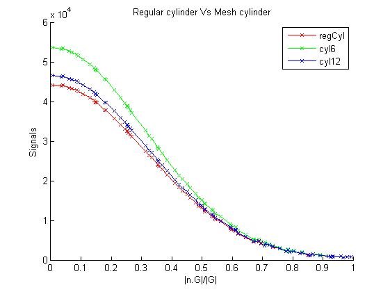
The code produces the following figure. We can observe that signal curve from cyl12 matches regCyl curve better than cyl6. This is well within our expectations as polygons with more vertices approximate circles better, and hence produces more accurate signals.

3.2  Undulating axons

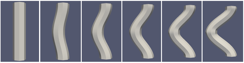
In this example, we will investigate the influence of axon undulation on diffusion MR signals. To model axons, we construct undulating cylinders with radius 3µm and height 25µm. Cylinders are along the z direction, and undulating in the x-direction with amplitudes ranging from 0µm to 5µm. There is no undulation in the y-direction. PLY files can be downloaded here and Paraview images as follows:

In this example, we use scheme myScheme2.scheme1, which contains three acquisitions with b-value = 1253.9 s/mm2, each only differs in gradient direction. We thus can investigate signal differences arise in x, y and z directions separately. The following commands run the simulations.

# specifies the scheme.
schemefile="myScheme2.scheme1"

# separations need to be greater than cylinder dimensions.
xsep=17E-6
ysep=7E-6
zsep=30E-6

# generates synthetic signals.
for Ax in 0 1 2 3 4 5
do
	file="unduAxon_Ax="${Ax}"E-6"
	plyfile=${file}.ply
	outputfile=${file}.Bfloat

	datasynth -walkers 1000 -tmax 1000 -p 0.0 -voxels 1 -initial intra -voxelsizefrac 1 -diffusivity 0.6E-9 \
-meshsep ${xsep} ${ysep} ${zsep} -schemefile ${schemefile} -substrate ply -plyfile ${plyfile} \
-outputfile ${outputfile}
done

We can then plot the synthetic signals using MATLAB.

% load signals.
for i = [0, 1, 2, 3, 4, 5]
    signalfName = sprintf('unduAxon_Ax=%dE-6.Bfloat', i);
    fid = fopen(signalfName, 'r', 'b');
    S(:, i+1) = fread(fid, 'float');
    fclose(fid);
end

% plot figure.
figure;
hold on;
plot(S(1, :), 'rx-');
plot(S(2, :), 'gx-');
plot(S(3, :), 'bx-');
xlabel('Amplitudes in x'); ylabel('Signals');
ylim([0,1000]);
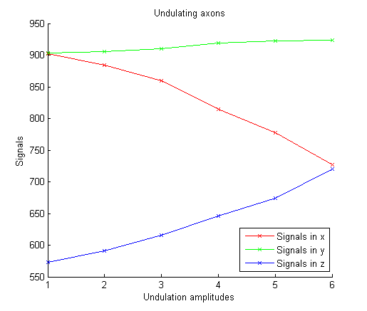
title('Undulating axons');
legend('Signals in x', 'Signals in y', 'Signals in z');

This produces the following figure. We can see that as amplitudes increase, signals decrease in x direction, increase in z direction, and remain nearly constant in y direction. Axon undulation thus influences diffusion MR signals, with larger signal decay in undulation direction while less decay in axon direction. Models assuming straight cylinders can be erroneous in the presence of axon undulation. We need to consider these effects when designing models.

Please note that the simulation can take a long time to initialise intracellular spins if the volume of the geometry is very small compared to the overall volume of the bounding box. Users could modify the code in Camino to initialise spins at the positions that they define as 'intra'.

References
1. Hall, M. G., Alexander, D. C. (2009). Convergence and Parameter Choice for Monte-Carlo Simulations of Diffusion MRI. IEEE Transactions on Medical Imaging 28(9), 1354-1364
2. Panagiotaki, E., Hall, M. G., Zhang, H., Siow, B., Lythgoe, M. F., Alexander, D. C. (2010). High-fidelity meshes from tissue samples for diffusion MRI simulations. MICCAI: 13(Pt 2), 404-411
3. Wang, T., Zhang, H., Hall, M. G., Alexander, D. C. (2013). The influence of macroscopic and microscopic fibre orientation dispersion on diffusion MR measurements: a Monte-Carlo simulation study. ISMRM.